

The Missing Guide to Diffusion Models (Part 1)
The Missing Guide to Diffusion Models (Part 1)

When I first set out to understand diffusion models, I kept running into the same frustrating pattern: short articles saying “they add noise to an image and then learn to denoise it,” with no real explanation of why that works, why it’s done step by step instead of once, or what the math is actually saying. On the other side of the spectrum, research papers dove into dense equations with shifting notations and an assumption that you already spoke the language fluently. There was nothing in between, nothing for someone who wanted to go beyond just downloading a pretrained model from Hugging Face, but wasn’t yet ready to reinvent the field.
After a year and a half of working with diffusion models, breaking them apart, implementing them, reading the papers in circles until they clicked, I want to write the series I wish I had back then. This will be a guided journey from the theory that makes diffusion models tick, through real implementations you can run and tinker with, and finally into the improvements that shaped the field, things like DDIM, classifier guidance, and beyond.
I’ll keep each article short enough to read in a sitting, but together they’ll form a complete roadmap: not just what diffusion models do, but why they work, and how to build on them yourself.
Prerequisites: basics of probability and statistics, and working familiarity with Python and PyTorch.
Roadmap:
- Diffusion Models: Intuition and the Big Picture
In this part, we’ll start with an intuition for what it means to generate data. We’ll also look at the difference between discriminative and generative models, explore the main families of generative approaches, introduce latent variable models and likelihood-based models and then conclude with a first look at diffusion models - Background: The Mathematical Foundations for Diffusion Models
Before touching diffusion models directly, we’ll build the mathematical foundation they rely on. This article introduces the Evidence Lower Bound (ELBO) and variational autoencoders. The goal is not to master VAEs for their own sake, but to use them to derive diffusion models. - Deriving Diffusion Models
With the background in place, we’ll derive diffusion models themselves. We’ll connect the parts and show why they work. - Building a Diffusion Model from scratch
Once the theory is clear, we’ll implement a basic diffusion model from scratch. We’ll train it on a small car dataset and observe how it gradually learns to reconstruct structure from pure noise. This part will focus on practical understanding. - Beyond the Basics: Modern Improvements
Finally, we’ll cover the main improvements and extensions that shaped modern diffusion models. This includes Conditional Diffusion, DDIM, Classifier Guidance, and Classifier-Free Guidance.
Part 1: Intuition and the Big Picture
1. Generating Samples: A Dice Analogy
Before we get into the mechanics of diffusion models, let’s take a step back and talk about what generative models actually try to do.
At their core, generative models have one main job: to generate new samples that look like they came from some real distribution of data.
Let’s start with something simple: rolling a fair six-sided dice.
If you’ve ever played a board game, you already know what this means: each face (1 through 6) has an equal chance of showing up.
Mathematically, we can write this as:
So if you wanted to generate samples from this distribution in other words, simulate dice rolls, that would be easy, right?
You could just write a small program that picks a number between 1 and 6 at random, each with equal probability.
Run it a hundred times, and you’ll get a list of numbers that look just like the outcomes of rolling a real fair dice.
But now imagine someone hands you a loaded dice.
This one doesn’t behave the same way, some numbers come up more often than others, and you have no idea how it’s rigged.
You can’t just assume each face has the same probability anymore. So what do you do?
To generate samples from this dice, you first need to understand how it behaves. So you start rolling it, over and over again, and record what you see. After enough rolls, you start to observe a pattern. Maybe 6 comes up more often than 1. Now, based on these observations, you try to estimate the underlying probability distribution P (x). Then, using that estimated probability, you can simulate new rolls of your loaded dice without ever touching the physical one again.
This, in essence, is what generative models do.
Given observed samples x from a distribution of interest, the goal of a generative model is to learn the true underlying data distribution p(x).
Once that distribution is learned, we can generate new samples that follow the same statistical patterns as the real data.
The key idea is to learn the hidden distribution behind real-world data, whether that data represents dice rolls, images of cats, or snippets of human speech.
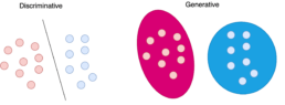
2. Discriminative vs Generative Models
In machine learning, models are often classified as either discriminative or generative, depending on what they aim to learn. This distinction comes from the probabilistic formulations used to build and train these models.
- Discriminative Models:
Discriminative models learn to predict a label y given an input data point x.
In other words, they learn the conditional probability distribution p(y|x).
The goal is to map data points to their correct labels. For example, a discriminative model trained to recognize digits in images learns how likely each digit is, given the image pixels. - Generative Models:
Generative models, try to learn a probability distribution over the data
points without external labels. They aim to learn p(x).
Our loaded dice analogy is an example: we observed outcomes x and tried to estimate the underlying probability distribution p(x) to generate new samples. - Conditional Generative Models:
Conditional generative models are still generative models. The difference is that they learn to generate data conditioned on additional information such as class labels, text prompts, or other context. They try to learn the probability distribution of the data x conditioned on the labels y. This is denoted as p(x|y). Here, y acts as a guiding signal, for example, generating an image of a “cat” when y=cat or a “dog” when y=dog.
3. Generative Models
The goal of generative models is to learn the probability density function of our data p(x). This probability density describes the behavior of our training data and allows us to generate new data by sampling from it. Ideally, we want our model to learn a density that matches the true data distribution.
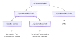
There are two broad classes of generative models:
- Explicit Density Models
These models can compute the density function p(x) explicitly.
After training, if we feed a data point x into the model, it can return its likelihood under the learned distribution.
Explicit models can be:
– Tractable: These models define a density that is computationally tractable, meaning we can directly calculate the likelihood for any given data point x. Examples include Autoregressive Models and Normalizing Flows.
– Approximate: These models still define an explicit density but parts of it are intractable to compute or optimize directly. They rely on approximation techniques to make training feasible. A common example is the Variational Autoencoder (VAE), which uses latent variables and optimizes a lower bound on the likelihood instead of the exact value (See part 2). - Implicit Density Models
Implicit density models do not compute p(x) directly. Instead, they are able to generate realistic samples from the data distribution without calculating the exact probability of each sample. The most common example is the Generative Adversarial Network (GAN), which learns to transform random noise into realistic data points through an adversarial training process.
Besides the distinction between implicit and explicit density models, generative models can also be categorized by the way they tackle the problem of learning the data distribution. Before moving to diffusion models, we’ll introduce two concepts that we’ll need later: latent variable models and likelihood-based models.
4. Latent Variable Models
To help us understand latent variable models, let’s start with a small analogy taken from Plato’s famous allegory of the cave.
Imagine a group of people who have lived their entire lives chained inside a dark cave. They cannot turn their heads, and all they can see are shadows flickering on the wall in front of them. Behind them, a fire burns, and objects pass between the fire and the prisoners, casting those shadows. To the prisoners, the shadows are reality and they have no idea that the real objects exist behind them. In the allegory, everything they observe is actually determined by higher-dimensional abstract concepts that they can never behold.

Just as the prisoners see only the shadows, we, in our everyday experience, see only the “projections” of deeper, hidden structures in the world. In the language of statistics and machine learning, these hidden structures are called latent variables. We can think of the data we observe as represented or generated by an associated unseen latent variable.
Even though the cave dwellers cannot see the real objects, they can reason about their shapes, sizes, and movements based on the shadows they observe. Similarly, we can try to infer the latent causes behind the data we see. In generative modeling, the goal is to learn a mapping between the latent space (the hidden causes) and the data space (the observable effects). Once we understand this mapping, we can even generate new “shadows”: new data points, that look real, even if we’ve never seen the original objects in their entirety.
One subtle but important point: unlike Plato’s cave, in machine learning we usually try to learn lower-dimensional latent representations. If the latent space were higher-dimensional than the data, the model would struggle to learn anything meaningful without strong assumptions. By compressing information into a smaller, latent space, we can often uncover semantically meaningful structures that explain the world around us.
Latent variable models aim to model the probability distribution with latent variables.
We can define seven basic terms:
- The marginal distribution p(x) is the distribution of the original data and it is the ultimate goal of the model. The marginal distribution tells us how possible it is to generate a data point.
- The prior distribution p(z) that models the behaviour of the latent variables
- The likelihood p(x|z) that defines how to map latent variables to the data points
- The joint distribution p(x, z) which is the multiplication of the likelihood and the prior and essentially describes our model.
- The posterior distribution p(z|x) which describes the latent variables that can be produced by a specific data point.
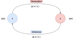
- Generation refers to the process of computing the data point x from the latent variable z. In essence, we move from the latent space to the actual data distribution. Mathematically this is represented by the likelihood p(x|z).
- Inference is the process of finding the latent variable z from the data point x and is formulated by the posterior distribution p(z|x) To generate a data point, we can sample z from p(z) and then sample the data point x from p(x|z).
5. Likelihood-based generative models.
As we discussed, the goal in generative modeling is to estimate the data distribution p(x). One of the classic statistical methods to do this is Maximum Likelihood Estimation (MLE). In statistics, MLE is a technique for estimating the parameters of a probability distribution using observed data. The idea is simple: choose the parameters that make the observed data most probable under the assumed model. To do this, we define a likelihood function, which measures how well a set of parameters explains the given data.
Formally, for observed data and parameters θ, the likelihood indicates how plausible different values of θ are, given the data. In other words, instead of asking “What is the probability of the data given the parameters?”, we ask “Given the data I observed, which parameters are most likely?”
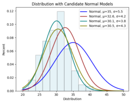
Imagine you collect random samples from a distribution and plot a histogram. It looks roughly like a normal distribution. A normal distribution is fully defined by two parameters:
- : the mean
- : the standard deviation
For every possible pair , you could ask:
“If the true distribution were , how likely is it that I would observe this exact dataset?”.
MLE provides a systematic way to answer that. You can visualize it as overlaying many normal curves on top of your histogram and selecting the one that best fits the data. This process is also known as fitting a parametric density model.
So the core idea is:
-
Define a likelihood function that tells us how likely our observed data is for a given set of parameters.
-
Find the parameters that maximize this likelihood, those are the best parameters for our distribution.
In practice, instead of maximizing the likelihood directly, we maximize the log-likelihood.
-
The logarithm is a monotonic function, it preserves the location of the maximum, so maximizing log-likelihood gives the same parameters as maximizing likelihood.
-
It simplifies the math dramatically
6. Diffusion models
Diffusion models are a new class of state-of-the-art generative models that generate diverse high-resolution images. Diffusion models solve a task similar to other generative model types, they attempt to approximate some probability distribution of a given domain q(x) and most importantly, provide a way to sample from that distribution x ∼ q(x).
The basic idea behind diffusion models is rather simple. They take the input image x0 and gradually add Gaussian noise to it through a series of T steps. We will call this the forward process. Afterward, a neural network is trained to recover the original data by reversing the noising process. By being able to model the reverse process, we can generate new data. This is the so-called reverse diffusion process or, in general, the sampling process of a generative model.
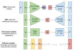
The figure above shows a high-level comparison between the architectures of GANs, VAEs, Flow-based models and Diffusion Models.
If you’re already familiar with GANs or VAEs, this might help you form an initial intuition for how diffusion models operate. If not, don’t worry. In the next articles, we’ll explore how diffusion models actually work in detail, step by step.
7. Where We Go from Here
In this first part, we built the groundwork for understanding diffusion models: what generative models do and how they differ from discriminative ones. We also explained latent variable, likelihood-based generative models and where diffusion models fit among VAEs and GANs.
Next, we’ll dig into the actual mechanics: how diffusion models connect to latent variable models, what the ELBO is, and why the “add noise, then denoise” idea works mathematically. From there, we’ll move on to building a simple diffusion model from scratch and explore the improvements that make modern variants so effective.
If you want to prepare, refresh some basic probability concepts and make sure you’re comfortable with the basics of Python and PyTorch.
And while you’re waiting for Part 2, feel free to check out my previous article, “A Refined Training Recipe for Fine-Grained Visual Classification”. You can also connect with me on LinkedIn, I’d love to hear your thoughts.
References:
[2] Lilian Weng. What are Diffusion Models?
[3] Calvin Luo. Understanding Diffusion Models: A Unified Perspective.