

The Missing Guide to Diffusion Models (Part 2)
The Missing Guide to Diffusion Models (Part 2)

Part 2: Background, The Mathematical Foundations for Diffusion Models
In the first part of this series, we built an intuition for generative modeling and placed diffusion models in the broader landscape of VAEs, GANs, and likelihood-based methods. We ended with a high-level idea: diffusion models gradually add Gaussian noise to data, step by step, and then learn to reverse that process.
The motivation for going all the way to noise is simple. If we can start from pure noise and reliably transform it into a realistic image, then we have a generative model. The forward noising process gives us a clean, well-defined starting point for sampling.
What’s less obvious is why this particular construction works.
Why does the noising happen gradually, instead of in a single step?
How does the model actually learn to denoise, and what training signal tells it that it is doing the right thing?
How does this correspond to learning a probability distribution at all?
Do we have mathematical guarantees that this process should work at all, rather than being a heuristic that just happens to work in practice?
These questions will be answered across the next two parts of the series. This second part is about setting up the necessary background. The third part will then focus entirely on diffusion models themselves. There, we will derive the forward noising process, the learned reverse dynamics, and the training objective in full detail. The goal here is not to memorize equations or reproduce derivations, but to build enough intuition to see the structure behind diffusion models. This is the level of understanding that lets you read papers, make sense of new variants as they appear, and reason about why certain design choices are made in the first place.
By the end of this part and the next, you should have a clear mental model for:
-
why the forward noising process is constructed the way it is,
-
why the reverse process can be learned at all,
-
and how all of this connects to likelihood-based training.
With that foundation in place, we’ll be ready to implement our first diffusion model from scratch.
Much of the intuition and probabilistic framing in this part and the next, is adapted from [1] Calvin Luo, Understanding Diffusion Models: A Unified Perspective. This article selectively borrows from that work and focuses on building intuition rather than presenting full mathematical rigor. If you’re looking for a more complete and formal treatment, the original paper is exceptionally well written and highly recommended.
1. Background: ELBO
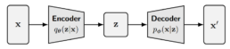
In Part 1, we explained that the goal of a generative model is to estimate the data density p(x). We also introduced latent variable models, where the observed data x is assumed to be generated with the help of unobserved latent variables z. In this setting, we can think of the model as described by a joint distribution: p(x,z).
Our goal is to learn the parameters of this distribution using the observed data. A natural approach is the Maximum Likelihood Estimation (MLE) we also presented in part 1, where we choose the parameters that maximize the likelihood of the observed data. The likelihood function measures the goodness of fit of a statistical model to a sample of data and it is formed from the joint probability distribution of the sample. Thus we want to to learn a model to maximize the likelihood p(x) of all observed x.
To connect the latent-variable model to the likelihood of the observed data, we marginalize out the latent variables:
We can also use the chain rule of probability:
\begin{equation} p(x) = \frac{p(x,z)}{p(z|x)} \end{equation}Directly computing and maximizing this likelihood is difficult, because it requires integrating over all possible latent variables z or having access to the true posterior distribution p(z/x). As discussed in Part 1, instead of maximizing the likelihood directly, we work with the log-likelihood, also called the evidence. The log-likelihood is easier to work with mathematically, but the core problem remains: the marginalization over z is still intractable.
To address this, we introduce a quantity called the Evidence Lower Bound (ELBO). The equation of the ELBO is:
\begin{equation} \mathbb{E}_{q_{\phi}(z|x)}\Biggl[\log{\frac{p(x,z)}{q_{\phi}(z|x)}}\Biggr] \end{equation}As its name suggests, the ELBO is a lower bound on the evidence:
\begin{equation}
\log{p(x)} \geq \mathbb{E}_{q_{\phi}(z|x)}\Biggl[\log{\frac{p(x,z)}{q_{\phi}(z|x)}}\Biggr]
\end{equation}
\text{Here, }q_{\phi}(z|x) \text{ is a parameterizable model that is trained to estimate the distribution over latent variables z given an observation }x \text{.}
\text{In other words, it is an approximation of the true posterior }p(z/x)\text{.}
Instead of optimizing the log-likelihood directly, we optimize a bound that we can work with. Maximizing the ELBO is a practical proxy with which to optimize a latent variable model.
Why is the Evidence Lower Bound (ELBO) a meaningful objective to optimize?
- Starting from Equation (1):
\begin{equation} \begin{split} \log p(x) & = \log \int p(x,z) \,dz \\ & = \log \int \frac{p(x,z) q_{\phi}(z|x)}{q_{\phi}(z|x)}\\ & = \log{\mathbb{E}_{q_{\phi}(z|x)}\Biggl[\frac{p(x,z)}{q_{\phi}(z|x)}\Biggr]} \text{\quad \quad \quad \quad \quad (Definition of Expectation)}\\ & \geq \mathbb{E}_{q_{\phi}(z|x)}\Biggl[\log{\frac{p(x,z)}{q_{\phi}(z|x)}}\Biggr] \text{\quad \quad \quad \quad \quad (Jensen's Inequality)} \end{split} \end{equation} - Using Equation 2:
\begin{equation} \begin{split} \log{p(x)} & = \log{p(x)} \int q_{\phi}(z|x) \,dz \\ & = \int q_{\phi}(z|x) (\log{p(x)})\,dz \\ & = \mathbb{E}_{q_{\phi}(z|x)}[\log{p(x)}] \text{\quad \quad \quad \quad \quad \quad \quad \quad \quad \quad \quad \quad \quad \quad \quad (Definition of Expectation)}\\ & = \mathbb{E}_{q_{\phi}(z|x)}\Biggl[\log{\frac{p(x,z)}{p(z|x)}}\Biggl] \text{\quad \quad \quad \quad \quad \quad \quad \quad \quad \quad \quad \quad \quad (Equation 2)}\\ & = \mathbb{E}_{q_{\phi}(z|x)}\Biggl[\log{\frac{p(x,z)q_{\phi}(z|x)}{p(z|x)q_{\phi}(z|x)}}\Biggl]\\ & = \mathbb{E}_{q_{\phi}(z|x)}\Biggl[\log{\frac{p(x,z)}{q_{\phi}(z|x)}}\Biggl] + \mathbb{E}_{q_{\phi}(z|z)}\Biggl[\log{\frac{q_{\phi}(z|x)}{p(z|x)}}\Biggl]\\ & = \mathbb{E}_{q_{\phi}(z|x)}\Biggl[\log{\frac{p(x,z)}{q_{\phi}(z|x)}}\Biggl] + D_{KL}(q_{\phi}(z|x) \parallel p(z|x)) \text{\quad \quad (Definition of KL Divergence)}\\ & \geq \mathbb{E}_{q_{\phi}(z|x)}\Biggl[\log{\frac{p(x,z)}{q_{\phi}(z|x)}}\Biggl] \text{\quad \quad \quad \quad \quad \quad \quad \quad \quad \quad \quad \quad \, (KL Divergence always $\geq 0$)} \end{split} \end{equation}
The last equation tells us that the evidence (the log-likelihood) can be decomposed into two terms: the Evidence Lower Bound (ELBO) and the KL divergence between the approximate posterior and the true posterior.
What does this mean in practice?
Recall that we introduced the latent variable z to capture the underlying structure that explains the observed data x. Our original objective, is to find the parameters of the generative model, denoted by θ, that maximize the log-likelihood log p(x) but it is difficult since we don’t have access to the true posterior distribution p(z/x). To make progress, we introduced an approximation parameterized by Φ. We want to optimize the parameters of our approximation to exactly match the true posterior distribution.
The KL divergence measures how close this approximation is to the true posterior distribution. Minimizing the KL divergence corresponds exactly to making this approximation better. In the idealized case where our approximation is expressive enough and optimization succeeds perfectly, the KL divergence goes to zero.
The key point is that maximizing the ELBO plays two different roles. The evidence term is a constant with respect to the variational parameters Φ. Since the ELBO and the KL divergence sum to this constant, any increase in the ELBO must be accompanied by a corresponding decrease in the KL divergence. As a result, maximizing the ELBO with respect to Φ implicitly minimizes the KL divergence. With respect to the model parameters θ, however, the situation is different. The ELBO is a lower bound on the evidence. Therefore, maximizing the ELBO with respect to θ is equivalent to optimizing the evidence itself.
This variational perspective: introducing latent variables, approximating their posterior, and optimizing a lower bound on the data likelihood, is the conceptual foundation that we will later build upon
2. Background: Variational Autoencoders (VAEs)
At the end of the previous section, we reached an important conclusion: one way to build a generative model with latent variables is to maximize the Evidence Lower Bound (ELBO) with respect to both the generative model parameters θ and the variational parameters ϕ. One model that relies on this idea is the variational autoencoder (VAE).
To understand VAEs, we need to address a subtle point that may not be intuitive to everyone: the posterior distribution is different for each data point x.
Consider a simple example. You observe the sum of two dice, which we call X, and the latent variable Z is the pair of individual dice values. If the observed sum is 2, the posterior distribution is trivial: the probability that both dice are 1 is 1, and the probability of any other outcome is 0. If the observed sum is 7, the posterior distribution is very different: several combinations such as (1,6), (2,5), and (3,4) all have non-zero probability. The shape of the distribution over latent variables depends entirely on the observed value of X.
Because the posterior is different for every data point, in principle we would need a separate set of variational parameters ϕ for each individual x. The key idea behind variational autoencoders is to avoid this problem by learning an inference network. Instead of directly optimizing variational parameters for each data point, we train a neural network that takes x as input and outputs the parameters of the variational posterior. This network is trained jointly with the generative model. The generative model (often called the decoder) has parameters θ, while the inference network (can be interpreted as an encoder) has parameters ϕ. Both are optimized simultaneously by maximizing the ELBO.
Equation 7 dissects the ELBO term further, to make the connection explicit:
The two terms in this decomposition play complementary roles. The first term, encourages the model to learn latent variables that retain the information necessary to reconstruct the observed data. In other words, it ensures that the learned latent representation is meaningful. The second term measures how similar the learned variational distribution is to a prior belief held over latent variables. Maximizing the ELBO therefore amounts to maximizing its first term and minimizing its second term.
Once the inference network is trained, computing the posterior for a new data point is straightforward: we simply pass the data through the encoder network.
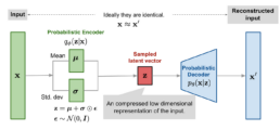
This architecture is called a variational autoencoder. It is autoencoder-like because data is mapped to a latent representation and then reconstructed back to itself through a bottleneck. It is variational because the latent representation is learned using variational inference. This probabilistic formulation encourages a smooth and continuous latent space, which is fundamentally different from the deterministic representations learned by standard autoencoders.
In practice, the encoder of a VAE is commonly chosen to model a multivariate Gaussian distribution with diagonal covariance, while the prior over latent variables is taken to be a standard multivariate Gaussian:
The KL divergence term of the ELBO can be computed analytically, and the first term can be approximated using a Monte Carlo estimate. Thus our objective can be rewritten as:
For each data point in the dataset, we sample latent variables \{z^{l}\}_{l=1}^{L} from the variational distribution q_{\phi}(z|x). However, this standard setup introduces a practical challenge: each z^{l} is generated through a stochastic sampling process, which is not directly differentiable. As a result, it is not possible to optimize the model parameters using standard gradient-based methods.
This problem is addressed by the reparameterization trick when q_{\phi}(z|x) is designed to model certain distributions, including the multivariate Gaussian. The idea is to express a random variable as a deterministic transformation of a noise variable that is independent of the model parameters. This simple but powerful reformulation allows gradients to flow through the sampling process.
To see how the reparameterization trick works in practice, consider a simple example. Suppose we want to draw samples from a normal distribution with arbitrary mean and variance: x \sim \mathcal{N}(\mu, \sigma^2).
Instead of sampling x directly from this distribution, we can rewrite this as a deterministic transformation of a standard normal variable: x = \mu + \sigma \epsilon, \text{with } \epsilon \sim \mathcal{N}(0, I).
Here, all the randomness is isolated in \epsilon, which is independent of the model parameters. The parameters \mu and \sigma now appear only in a deterministic transformation. This reformulation is mathematically equivalent to sampling from \mathcal{N}(\mu, \sigma^2), but it has a crucial practical advantage: gradients can flow through \muand \sigma during backpropagation.
In a variational autoencoder, the same idea is applied to the latent variable z. Recall that the encoder outputs the parameters of a Gaussian distribution: q_\phi(z \mid x) = \mathcal{N}\bigl(z; \mu_\phi(x), \sigma_\phi^2(x) I \bigr). Instead of sampling z directly from this distribution, we write: z = \mu_\phi(x) + \sigma_\phi(x) \odot \epsilon, \text{with } \epsilon \sim \mathcal{N}(0, I), where \odot denotes element-wise multiplication.
In this formulation, z is a deterministic function of the input x, the encoder parameters \phi, and an auxiliary noise variable \epsilon. The stochasticity is fully captured by \epsilon, which is independent of the network parameters. This allows us to compute gradients of the ELBO with respect to both \phiand \theta using standard gradient-based optimization.
The VAE therefore combines two key ideas:
-
Monte Carlo estimation to approximate expectations, and
-
the reparameterization trick to make those estimates differentiable.
After training, generation is straightforward. We sample directly from the prior over latent variables, z \sim p(z) and pass the sampled latent variable through the decoder. If training has succeeded, decoding samples from this simple Gaussian prior produces realistic data points in the original data space.
2. Background: From Variational Autoencoders to Hierarchical Variational Autoencoders
So far, we have studied the variational autoencoder as a latent variable model with a single layer of latent variables. We will now introduce an idea that generalizes this formulation. Instead of assuming that the data is generated from one latent variable, we allow multiple layers of latent variables, arranged hierarchically. In this setting, latent variables themselves are interpreted as generated from higher-level, more abstract latent variables. This leads to what is known as a Hierarchical Variational Autoencoder (HVAE).
In an HVAE with T hierarchical levels, each latent variable is, in general, allowed to condition on all previous latent variables in the hierarchy.
In this work, however, we focus on a particular structured case that we refer to as a Markovian Hierarchical VAE (MHVAE). In an MHVAE, the generative process forms a Markov chain. Each transition down the hierarchy is Markovian, meaning that decoding each latent variable z_t depends only on the latent variable directly above it, z_{t+1}. Intuitively, this structure can be viewed as stacking multiple VAEs on top of one another.
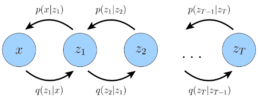
Mathematically, we represent the joint distribution and the posterior of a Markovian HVAE as:
Then, the ELBO can be extended to:
\begin{equation} = \log \int \frac{p(x, z_{1:T}) q_\phi(z_{1:T} \mid x)}{q_\phi(z_{1:T} \mid x)} , dz_{1:T} \end{equation}
\begin{equation} = \log \mathbb{E}_{q_\phi(z_{1:T} \mid x)} \left[ \frac{p(x, z_{1:T})}{q_\phi(z_{1:T} \mid x)} \right] \end{equation}
\begin{equation} \geq \mathbb{E}_{q_\phi(z_{1:T} \mid x)} \log \left[ \frac{p(x, z_{1:T})}{q_\phi(z_{1:T} \mid x)} \right] \end{equation}
We can substitute the joint distribution (Equation 11) and the posterior (Equation 12) into Equation 16 to obtain an alternative form:
In this setting, generation becomes a sequential process: we sample from a simple prior at the top of the hierarchy and progressively transform it into data through a chain of conditional distributions. This perspective will turn out to be crucial, because diffusion models can be understood as a very particular instantiation of this framework.
3. Where We Go from Here
In this article, we built the mathematical foundation necessary to understand diffusion models. We derived the Evidence Lower Bound (ELBO), explored variational autoencoders, and then generalized them to hierarchical and Markovian variational autoencoders. Along the way, we saw how maximizing the ELBO allows us to train generative models even when the true posterior is intractable.
In the next part, we will see that diffusion models are a very specific and carefully constructed instance of a Markovian Hierarchical VAE and the diffusion training objective will emerge naturally from the ELBO we derived here. Once that connection is fully clear, we will move from theory to practice. In Part 4, we will implement a diffusion model from scratch, translating every mathematical component into working PyTorch code. At that point, the entire picture will come together.
References:
[1] Calvin Luo. Understanding Diffusion Models: A Unified Perspective.
[2] Lilian Weng. From Autoencoder to Beta-VAE.
[3] Chieh-Hsin Lai et al. The Principles of Diffusion Models.
The Missing Guide to Diffusion Models (Part 1)
The Missing Guide to Diffusion Models (Part 1)
When I first set out to understand diffusion models, I kept running into the same frustrating pattern: short articles saying “they add noise to an image and then learn to denoise it,” with no real explanation of why that works, why it’s done step by step instead of once, or what the math is actually saying. On the other side of the spectrum, research papers dove into dense equations with shifting notations and an assumption that you already spoke the language fluently. There was nothing in between, nothing for someone who wanted to go beyond just downloading a pretrained model from Hugging Face, but wasn’t yet ready to reinvent the field.
After a year and a half of working with diffusion models, breaking them apart, implementing them, reading the papers in circles until they clicked, I want to write the series I wish I had back then. This will be a guided journey from the theory that makes diffusion models tick, through real implementations you can run and tinker with, and finally into the improvements that shaped the field, things like DDIM, classifier guidance, and beyond.
I’ll keep each article short enough to read in a sitting, but together they’ll form a complete roadmap: not just what diffusion models do, but why they work, and how to build on them yourself.
Prerequisites: basics of probability and statistics, and working familiarity with Python and PyTorch.
Roadmap:
- Diffusion Models: Intuition and the Big Picture
In this part, we’ll start with an intuition for what it means to generate data. We’ll also look at the difference between discriminative and generative models, explore the main families of generative approaches, introduce latent variable models and likelihood-based models and then conclude with a first look at diffusion models - Background: The Mathematical Foundations for Diffusion Models
Before touching diffusion models directly, we’ll build the mathematical foundation they rely on. This article introduces the Evidence Lower Bound (ELBO) and variational autoencoders. The goal is not to master VAEs for their own sake, but to use them to derive diffusion models. - Deriving Diffusion Models
With the background in place, we’ll derive diffusion models themselves. We’ll connect the parts and show why they work. - Building a Diffusion Model from scratch
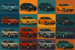
Once the theory is clear, we’ll implement a basic diffusion model from scratch. We’ll train it on a small car dataset and observe how it gradually learns to reconstruct structure from pure noise. This part will focus on practical understanding. - Beyond the Basics: Modern Improvements
Finally, we’ll cover the main improvements and extensions that shaped modern diffusion models. This includes Conditional Diffusion, DDIM, Classifier Guidance, and Classifier-Free Guidance.
Part 1: Intuition and the Big Picture
1. Generating Samples: A Dice Analogy
Before we get into the mechanics of diffusion models, let’s take a step back and talk about what generative models actually try to do.
At their core, generative models have one main job: to generate new samples that look like they came from some real distribution of data.
Let’s start with something simple: rolling a fair six-sided dice.
If you’ve ever played a board game, you already know what this means: each face (1 through 6) has an equal chance of showing up.
Mathematically, we can write this as:
So if you wanted to generate samples from this distribution in other words, simulate dice rolls, that would be easy, right?
You could just write a small program that picks a number between 1 and 6 at random, each with equal probability.
Run it a hundred times, and you’ll get a list of numbers that look just like the outcomes of rolling a real fair dice.
But now imagine someone hands you a loaded dice.
This one doesn’t behave the same way, some numbers come up more often than others, and you have no idea how it’s rigged.
You can’t just assume each face has the same probability anymore. So what do you do?
To generate samples from this dice, you first need to understand how it behaves. So you start rolling it, over and over again, and record what you see. After enough rolls, you start to observe a pattern. Maybe 6 comes up more often than 1. Now, based on these observations, you try to estimate the underlying probability distribution P (x). Then, using that estimated probability, you can simulate new rolls of your loaded dice without ever touching the physical one again.
This, in essence, is what generative models do.
Given observed samples x from a distribution of interest, the goal of a generative model is to learn the true underlying data distribution p(x).
Once that distribution is learned, we can generate new samples that follow the same statistical patterns as the real data.
The key idea is to learn the hidden distribution behind real-world data, whether that data represents dice rolls, images of cats, or snippets of human speech.
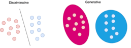
2. Discriminative vs Generative Models
In machine learning, models are often classified as either discriminative or generative, depending on what they aim to learn. This distinction comes from the probabilistic formulations used to build and train these models.
- Discriminative Models:
Discriminative models learn to predict a label y given an input data point x.
In other words, they learn the conditional probability distribution p(y|x).
The goal is to map data points to their correct labels. For example, a discriminative model trained to recognize digits in images learns how likely each digit is, given the image pixels. - Generative Models:
Generative models, try to learn a probability distribution over the data
points without external labels. They aim to learn p(x).
Our loaded dice analogy is an example: we observed outcomes x and tried to estimate the underlying probability distribution p(x) to generate new samples. - Conditional Generative Models:
Conditional generative models are still generative models. The difference is that they learn to generate data conditioned on additional information such as class labels, text prompts, or other context. They try to learn the probability distribution of the data x conditioned on the labels y. This is denoted as p(x|y). Here, y acts as a guiding signal, for example, generating an image of a “cat” when y=cat or a “dog” when y=dog.
3. Generative Models
The goal of generative models is to learn the probability density function of our data p(x). This probability density describes the behavior of our training data and allows us to generate new data by sampling from it. Ideally, we want our model to learn a density that matches the true data distribution.
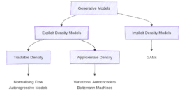
There are two broad classes of generative models:
- Explicit Density Models
These models can compute the density function p(x) explicitly.
After training, if we feed a data point x into the model, it can return its likelihood under the learned distribution.
Explicit models can be:
– Tractable: These models define a density that is computationally tractable, meaning we can directly calculate the likelihood for any given data point x. Examples include Autoregressive Models and Normalizing Flows.
– Approximate: These models still define an explicit density but parts of it are intractable to compute or optimize directly. They rely on approximation techniques to make training feasible. A common example is the Variational Autoencoder (VAE), which uses latent variables and optimizes a lower bound on the likelihood instead of the exact value (See part 2). - Implicit Density Models
Implicit density models do not compute p(x) directly. Instead, they are able to generate realistic samples from the data distribution without calculating the exact probability of each sample. The most common example is the Generative Adversarial Network (GAN), which learns to transform random noise into realistic data points through an adversarial training process.
Besides the distinction between implicit and explicit density models, generative models can also be categorized by the way they tackle the problem of learning the data distribution. Before moving to diffusion models, we’ll introduce two concepts that we’ll need later: latent variable models and likelihood-based models.
4. Latent Variable Models
To help us understand latent variable models, let’s start with a small analogy taken from Plato’s famous allegory of the cave.
Imagine a group of people who have lived their entire lives chained inside a dark cave. They cannot turn their heads, and all they can see are shadows flickering on the wall in front of them. Behind them, a fire burns, and objects pass between the fire and the prisoners, casting those shadows. To the prisoners, the shadows are reality and they have no idea that the real objects exist behind them. In the allegory, everything they observe is actually determined by higher-dimensional abstract concepts that they can never behold.

Just as the prisoners see only the shadows, we, in our everyday experience, see only the “projections” of deeper, hidden structures in the world. In the language of statistics and machine learning, these hidden structures are called latent variables. We can think of the data we observe as represented or generated by an associated unseen latent variable.
Even though the cave dwellers cannot see the real objects, they can reason about their shapes, sizes, and movements based on the shadows they observe. Similarly, we can try to infer the latent causes behind the data we see. In generative modeling, the goal is to learn a mapping between the latent space (the hidden causes) and the data space (the observable effects). Once we understand this mapping, we can even generate new “shadows”: new data points, that look real, even if we’ve never seen the original objects in their entirety.
One subtle but important point: unlike Plato’s cave, in machine learning we usually try to learn lower-dimensional latent representations. If the latent space were higher-dimensional than the data, the model would struggle to learn anything meaningful without strong assumptions. By compressing information into a smaller, latent space, we can often uncover semantically meaningful structures that explain the world around us.
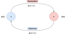
Latent variable models aim to model the probability distribution with latent variables.
We can define seven basic terms:
- The marginal distribution p(x) is the distribution of the original data and it is the ultimate goal of the model. The marginal distribution tells us how possible it is to generate a data point.
- The prior distribution p(z) that models the behaviour of the latent variables
- The likelihood p(x|z) that defines how to map latent variables to the data points
- The joint distribution p(x, z) which is the multiplication of the likelihood and the prior and essentially describes our model.
- The posterior distribution p(z|x) which describes the latent variables that can be produced by a specific data point.
- Generation refers to the process of computing the data point x from the latent variable z. In essence, we move from the latent space to the actual data distribution. Mathematically this is represented by the likelihood p(x|z).
- Inference is the process of finding the latent variable z from the data point x and is formulated by the posterior distribution p(z|x) To generate a data point, we can sample z from p(z) and then sample the data point x from p(x|z).
5. Likelihood-based generative models.
As we discussed, the goal in generative modeling is to estimate the data distribution p(x). One of the classic statistical methods to do this is Maximum Likelihood Estimation (MLE). In statistics, MLE is a technique for estimating the parameters of a probability distribution using observed data. The idea is simple: choose the parameters that make the observed data most probable under the assumed model. To do this, we define a likelihood function, which measures how well a set of parameters explains the given data.
Formally, for observed data and parameters θ, the likelihood indicates how plausible different values of θ are, given the data. In other words, instead of asking “What is the probability of the data given the parameters?”, we ask “Given the data I observed, which parameters are most likely?”
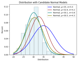
Imagine you collect random samples from a distribution and plot a histogram. It looks roughly like a normal distribution. A normal distribution is fully defined by two parameters:
- : the mean
- : the standard deviation
For every possible pair , you could ask:
“If the true distribution were , how likely is it that I would observe this exact dataset?”.
MLE provides a systematic way to answer that. You can visualize it as overlaying many normal curves on top of your histogram and selecting the one that best fits the data. This process is also known as fitting a parametric density model.
So the core idea is:
-
Define a likelihood function that tells us how likely our observed data is for a given set of parameters.
-
Find the parameters that maximize this likelihood, those are the best parameters for our distribution.
In practice, instead of maximizing the likelihood directly, we maximize the log-likelihood.
-
The logarithm is a monotonic function, it preserves the location of the maximum, so maximizing log-likelihood gives the same parameters as maximizing likelihood.
-
It simplifies the math dramatically
6. Diffusion models
Diffusion models are a new class of state-of-the-art generative models that generate diverse high-resolution images. Diffusion models solve a task similar to other generative model types, they attempt to approximate some probability distribution of a given domain q(x) and most importantly, provide a way to sample from that distribution x ∼ q(x).
The basic idea behind diffusion models is rather simple. They take the input image x0 and gradually add Gaussian noise to it through a series of T steps. We will call this the forward process. Afterward, a neural network is trained to recover the original data by reversing the noising process. By being able to model the reverse process, we can generate new data. This is the so-called reverse diffusion process or, in general, the sampling process of a generative model.
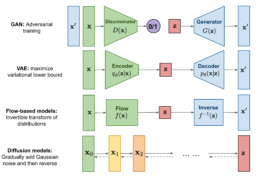
The figure above shows a high-level comparison between the architectures of GANs, VAEs, Flow-based models and Diffusion Models.
If you’re already familiar with GANs or VAEs, this might help you form an initial intuition for how diffusion models operate. If not, don’t worry. In the next articles, we’ll explore how diffusion models actually work in detail, step by step.
7. Where We Go from Here
In this first part, we built the groundwork for understanding diffusion models: what generative models do and how they differ from discriminative ones. We also explained latent variable, likelihood-based generative models and where diffusion models fit among VAEs and GANs.
Next, we’ll dig into the actual mechanics: how diffusion models connect to latent variable models, what the ELBO is, and why the “add noise, then denoise” idea works mathematically. From there, we’ll move on to building a simple diffusion model from scratch and explore the improvements that make modern variants so effective.
If you want to prepare, refresh some basic probability concepts and make sure you’re comfortable with the basics of Python and PyTorch.
And while you’re waiting for Part 2, feel free to check out my previous article, “A Refined Training Recipe for Fine-Grained Visual Classification”. You can also connect with me on LinkedIn, I’d love to hear your thoughts.
References:
[2] Lilian Weng. What are Diffusion Models?
[3] Calvin Luo. Understanding Diffusion Models: A Unified Perspective.
A Refined Training Recipe for Fine-Grained Visual Classification
A Refined Training Recipe for Fine-Grained Visual Classification

For the past year, my research at Multitel has focused on fine-grained visual classification (FGVC). Specifically, I worked on building a robust car classifier that can work in real-time on edge devices. This post is part of what may become a small series of reflections on this experience. I’m writing to share some of the lessons I learned but also to organize and compound what I’ve learned. At the same time, I hope this gives a sense of the kind of high-level engineering and applied research we do at Multitel, work that blends academic rigor with real-world constraints. Whether you’re a fellow researcher, a curious engineer, or someone considering joining our team, I hope this post offers both insight and inspiration.
1. The problem:
We needed a system that could identify specific car models, not just “this is a BMW,” but which BMW model and year. And it needed to run in real time on resource-constrained edge devices alongside other models. This kind of task falls under what’s known as fine-grained visual classification (FGVC).
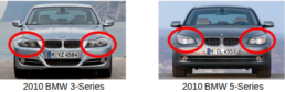
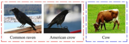
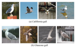
FGVC aims to recognize images belonging to multiple subordinate categories of a super-category (e.g. species of animals / plants, models of cars etc). The difficulty lies with understanding fine-grained visual differences that sufficiently discriminate between objects that are highly similar in overall appearance but differ in fine-grained features [2].
What makes FGVC particularly tricky?
- Small inter-class variation: The visual differences between classes can be extremely subtle.
- Large intra-class variation: At the same time, instances within the same class may vary greatly due to changes in lighting, pose, background, or other environmental factors.
- The subtle visual differences can be easily overwhelmed by the other factors such as poses and viewpoints.
- Long-tailed distributions: Datasets typically have a few classes with many samples and many classes with very few examples. For example, you might have only a couple of images of a rare spider species found in a remote region, while common species have thousands of images. This imbalance makes it difficult for models to learn equally well across all categories.
2. The landscape:
When we first started tackling this problem, we naturally turned to literature. We dove into academic papers, examined benchmark datasets, and explored state-of-the-art FGVC methods. And at first, the problem seemed far more complicated than it actually turned out to be, at least in our specific context.
FGVC has been actively researched for years, and there’s no shortage of approaches that introduce increasingly complex architectures and pipelines. Many early works, for example, proposed two-stage models: a localization subnetwork would first identify discriminative object parts, and then a second network would classify based on those parts. Others focused on custom loss functions, high-order feature interactions, or label dependency modeling using hierarchical structures.
All of these methods were designed to tackle the subtle visual distinctions that make FGVC so challenging. If you’re curious about the evolution of these approaches, Wei et al [2]. provide a solid survey that covers many of them in depth.
When we looked closer at recent benchmark results (archived from Papers with Code), many of the top-performing solutions were based on transformer architectures. These models often reached state-of-the-art accuracy, but with little to no discussion of inference time or deployment constraints. Given our requirements, we were fairly certain that these models wouldn’t hold up in real-time on an edge device already running multiple models in parallel.
At the time of this work, the best reported result on Stanford Cars was 97.1% accuracy, achieved by CMAL-Net.
3. Our approach:
Instead of starting with the most complex or specialized solutions, we took the opposite approach: Could a model that we already knew would meet our real-time and deployment constraints perform well enough on the task? Specifically, we asked whether a solid general-purpose architecture could get us close to the performance of more recent, heavier models, if trained properly.
That line of thinking led us to a paper by Ross Wightman et al., “ResNet Strikes Back: An Improved Training Procedure in Timm.” In it, Wightman makes a compelling argument: most new architectures are trained using the latest advancements and techniques but then compared against older baselines trained with outdated recipes. Wightman argues that ResNet-50, which is frequently used as a benchmark, is often not given the benefit of these modern improvements. His paper proposes a refined training procedure and shows that, when trained properly, even a vanilla ResNet-50 can achieve surprisingly strong results, including on several FGVC benchmarks.
With these constraints and goals in mind, we set out to build our own strong, reusable training procedure, one that could deliver high performance on FGVC tasks without relying on architecture-specific tricks. The idea was simple: start with a known, efficient backbone like ResNet-50 and focus entirely on improving the training pipeline rather than modifying the model itself. That way, the same recipe could later be applied to other architectures with minimal adjustments.
We began collecting ideas, techniques, and training refinements from across several sources, compounding best practices into a single, cohesive pipeline. In particular, we drew from four key resources:
- Bag of Tricks for Image Classification with Convolutional Neural Networks (He et al.)
- Compounding the Performance Improvements of Assembled Techniques in a Convolutional Neural Network (Lee et al.)
- ResNet Strikes Back: An Improved Training Procedure in Timm (Wightman et al.)
- How to Train State-of-the-Art Models Using TorchVision’s Latest Primitives (Vryniotis)
Our goal was to create a robust training pipeline that didn’t rely on model-specific tweaks. That meant focusing on techniques that are broadly applicable across architectures.
To test and validate our training pipeline, we used the Stanford Cars dataset [9], a widely used fine-grained classification benchmark that closely aligns with our real-world use case. The dataset contains 196 car categories and 16,185 images, all taken from the rear to emphasize subtle inter-class differences. The data is nearly evenly split between 8,144 training images and 8,041 testing images. To simulate our deployment scenario, where the classification model operates downstream of an object detection system, we crop each image to its annotated bounding box before training and evaluation.
While the original hosting site for the dataset is no longer available, it remains accessible via curated repositories such as Kaggle, and Huggingface. The dataset is distributed under the BSD-3-Clause license, which permits both commercial and non-commercial use. In this work, it was used solely in a research context to produce the results presented here.

Building the Recipe
What follows is the distilled training recipe we arrived at, built through experimentation, iteration, and careful aggregation of ideas from the works mentioned above. The idea is to show that by simply applying modern training best practices, without any architecture-specific hacks, we could get a general-purpose model like ResNet-50 to perform competitively on a fine-grained benchmark.
We’ll start with a vanilla ResNet-50 trained using a basic setup and progressively introduce improvements, one step at a time.
With each technique, we’ll report:
- The individual performance gain
- The cumulative gain when added to the pipeline
While many of the techniques used are likely familiar, our intent is to highlight how powerful they can be when compounded intentionally. Benchmarks often obscure this by comparing new architectures trained with the latest advancements to old baselines trained with outdated recipes. Here, we want to flip that and show what’s possible with a carefully tuned recipe applied to a widely available, efficient backbone.
We also recognize that many of these techniques interact with each other. So, in practice, we tuned some combinations through greedy or grid search to account for synergies and interdependencies.
The Base Recipe:
Before diving into optimizations, we start with a clean, simple baseline.
We train a ResNet-50 model pretrained on ImageNet using the Stanford Cars dataset. Each model is trained for 600 epochs on a single RTX 4090 GPU, with early stopping based on validation accuracy using a patience of 200 epochs.
We use:
- Nesterov Accelerated Gradient (NAG) for optimization
- Learning rate: 0.01
- Batch size: 32
- Momentum: 0.9
- Loss function: Cross-entropy
All training and validation images are cropped to their bounding boxes and resized to 224×224 pixels. We start with the same standard augmentation policy as in [5].
Here’s a summary of the base training configuration and its performance:
| Model | Pretrain | Optimizer | Learning rate | Momentum | Batch size | Loss function | Image size | Epochs | Patience | Augmentation | Accuracy |
|---|---|---|---|---|---|---|---|---|---|---|---|
| ResNet50 | ImageNet | NAG | 0.01 | 0.9 | 32 | Crossentropy Loss | 224x224 | 600 | 200 | Standard | 88.22% |
We fix the random seed across runs to ensure reproducibility and reduce variance between experiments. To assess the true effect of a change in the recipe, we follow best practices and average results over multiple runs (typically 3 to 5).
We’ll now build on top of this baseline step-by-step, introducing one technique at a time and tracking its impact on accuracy. The goal is to isolate what each component contributes and how they compound when applied together.
Large batch training:
In mini-batch SGD, gradient descending is a random process because the examples are randomly selected in each batch. Increasing the batch size does not change the expectation of the stochastic gradient but reduces its variance. Using large batch size, however, may slow down the training progress. For the same number of epochs, training with a large batch size results in a model with degraded validation accuracy compared to the ones trained with smaller batch sizes.
He et al [5] argues that linearly increasing the learning rate with the batch size works empirically for ResNet-50 training.
To improve both the accuracy and the speed of our training we change the batch size to 128 and the learning rate to 0.1. We add a StepLR scheduler that decays the learning rate of each parameter group by 0.1 every 30 epochs.
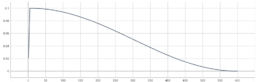
Learning rate warmup:
Since at the beginning of the training all parameters are typically random values using a too large learning rate may result in numerical instability.
In the warmup heuristic, we use a small learning rate at the beginning and then switch back to the initial learning rate when the training process is stable. We use a gradual warmup strategy that increases the learning rate from 0 to the initial learning rate linearly.
We add a linear warmup strategy for 5 epochs.
| Model | Pretrain | Optimizer | Learning rate | Momentum | Batch size | Loss function | Image size | Epochs | Patience | |
|---|---|---|---|---|---|---|---|---|---|---|
| ResNet50 | ImageNet | NAG | 0.1 | 0.9 | 128 | Crossentropy Loss | 224x224 | 600 | 200 | |
| Augmentation | Scheduler | Scheduler step size | Scheduler Gamma | Warmup Method | Warmup epochs | Warmup decay | Accuracy | Incremental Improvement | Absolute Improvement | |
| Standard | StepLR | 30 | 0.1 | Linear | 5 | 0.01 | 89.21 | +0.99 | +0.99 | |
Trivial Augment:
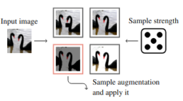
To explore the impact of stronger data augmentation, we replaced the baseline augmentation with TrivialAugment. Trivial Augment works as follows. It takes an image x and a set of augmentations A as input. It then simply samples an augmentation from A uniformly at random and applies this augmentation to the given image x with a strength m, sampled uniformly at random from the set of possible strengths {0, . . . , 30}, and returns the augmented image.
What makes TrivialAugment especially attractive is that it’s completely parameter-free, it doesn’t require search or tuning, making it a simple yet effective drop-in replacement that reduces experimental complexity.
While it may seem counterintuitive that such a generic and randomized strategy would outperform augmentations specifically tailored to the dataset or more sophisticated automated augmentation methods, we tried a variety of alternatives, and TrivialAugment consistently delivered strong results across runs. Its simplicity, stability, and surprisingly high effectiveness make it a compelling default choice.
| Model | Pretrain | Optimizer | Learning rate | Momentum | Batch size | Loss function | Image size | Epochs | Patience |
|---|---|---|---|---|---|---|---|---|---|
| ResNet50 | ImageNet | NAG | 0.1 | 0.9 | 128 | Crossentropy Loss | 224x224 | 600 | 200 |
| Scheduler | Scheduler step size | Scheduler Gamma | Warmup Method | Warmup epochs | Warmup decay | Augmentation | Accuracy | Incremental Improvement | Absolute Improvement |
| StepLR | 30 | 0.1 | Linear | 5 | 0.01 | TrivialAugment | 92.66 | +3.45 | +4.44 |
Cosine Learning Rate Decay:
Next, we explored modifying the learning rate schedule. We switched to a cosine annealing strategy, which decreases the learning rate from the initial value to 0 by following the cosine function. A big advantage of cosine is that there are no hyper-parameters to optimize, which cuts down again our search space.
| Model | Pretrain | Optimizer | Learning rate | Momentum | Batch size | Loss function | Image size | Epochs | Patience |
|---|---|---|---|---|---|---|---|---|---|
| ResNet50 | ImageNet | NAG | 0.1 | 0.9 | 128 | Crossentropy Loss | 224x224 | 600 | 200 |
| Scheduler | Scheduler step size | Scheduler Gamma | Warmup Method | Warmup epochs | Warmup decay | Augmentation | Accuracy | Incremental Improvement | Absolute Improvement |
| Cosine | - | - | Linear | 5 | 0.01 | TrivialAugment | 93.22 | +0.56 | +5 |
Label Smoothing:
A good technique to reduce overfitting is to stop the model from becoming overconfident. This can be achieved by softening the ground truth using Label Smoothing. The idea is to change the construction of the true label to:
There is a single parameter which controls the degree of smoothing (the higher the stronger) that we need to specify. We used a smoothing factor of ε = 0.1, which is the standard value proposed in the original paper and widely adopted in the literature.
Interestingly, we found empirically that adding label smoothing reduced gradient variance during training. This allowed us to safely increase the learning rate without destabilizing training. As a result, we increased the initial learning rate from 0.1 to 0.4
| Model | Pretrain | Optimizer | Learning rate | Momentum | Batch size | Loss function | Image size |
|---|---|---|---|---|---|---|---|
| ResNet50 | ImageNet | NAG | 0.4 | 0.9 | 128 | Crossentropy Loss | 224x224 |
| Epochs | Patience | Scheduler | Scheduler step size | Scheduler Gamma | Warmup Method | Warmup epochs | Warmup decay |
| 600 | 200 | Cosine | - | - | Linear | 5 | 0.01 |
| Augmentation | Label Smoothing | Accuracy | Incremental Improvement | Absolute Improvement | |||
| TrivialAugment | 0.1 | 94.5 | +1.28 | +6.28 |
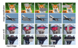
Random Erasing:
As an additional form of regularization, we introduced Random Erasing into the training pipeline. This technique randomly selects a rectangular region within an image and replaces its pixels with random values, with a fixed probability.
Often paired with Automatic Augmentation methods, it usually yields additional improvements in accuracy due to its regularization effect. We added Random Erasing with a probability of 0.1.
| Model | Pretrain | Optimizer | Learning rate | Momentum | Batch size | Loss function | Image size |
|---|---|---|---|---|---|---|---|
| ResNet50 | ImageNet | NAG | 0.4 | 0.9 | 128 | Crossentropy Loss | 224x224 |
| Epochs | Patience | Scheduler | Scheduler step size | Scheduler Gamma | Warmup Method | Warmup epochs | Warmup decay |
| 600 | 200 | Cosine | - | - | Linear | 5 | 0.01 |
| Augmentation | Label Smoothing | Random Erasing | Accuracy | Incremental Improvement | Absolute Improvement | ||
| TrivialAugment | 0.1 | 0.1 | 94.93 | +0.43 | +6.71 |
Exponential Moving Average (EMA):
Training a neural network using mini batches introduces noise and less accurate gradients when gradient descent updates the model parameters between batches. Exponential moving average is used in training deep neural networks to improve their stability and generalization.
Instead of just using the raw weights that are directly learned during training, EMA maintains a running average of the model weights which are then updated at each training step using a weighted average of the current weights and the previous EMA values.
Specifically, at each training step, the EMA weights are updated using:
where θ are the current model weights and α is a decay factor controlling how much weight is given to the past.
By evaluating the EMA weights rather than the raw ones at test time, we found improved consistency in performance across runs, especially in the later stages of training.
| Model | Pretrain | Optimizer | Learning rate | Momentum | Batch size | Loss function | Image size |
|---|---|---|---|---|---|---|---|
| ResNet50 | ImageNet | NAG | 0.4 | 0.9 | 128 | Crossentropy Loss | 224x224 |
| Epochs | Patience | Scheduler | Scheduler step size | Scheduler Gamma | Warmup Method | Warmup epochs | Warmup decay |
| 600 | 200 | Cosine | - | - | Linear | 5 | 0.01 |
| Augmentation | Label Smoothing | Random Erasing | EMA Steps | EMA Decay | Accuracy | Incremental Improvement | Absolute Improvement |
| TrivialAugment | 0.1 | 0.1 | 32 | 0.994 | 94.93 | 0 | +6.71 |
We tested EMA in isolation, and found that it led to notable improvements in both training stability and validation performance. But when we integrated EMA into the full recipe alongside other techniques, it did not provide further improvement. The results appeared to plateau, suggesting that most of the gains had already been captured by the other components.
Because our goal is to develop a general-purpose training recipe rather than one overly tailored to a single dataset, we chose to keep EMA in the final setup. Its benefits may be more pronounced in other conditions, and its low overhead makes it a safe inclusion.
Optimizations we tested but didn’t adopt:
We also explored a range of additional techniques that are commonly effective in other image classification tasks, but found that they either did not lead to significant improvements or, in some cases, slightly regressed performance on the Stanford Cars dataset:
- Weight Decay: Adds L2 regularization to discourage large weights during training. We experimented extensively with weight decay in our use case, but it consistently regressed performance.
- Cutmix/Mixup: Cutmix replaces random patches between images and mixes the corresponding labels. Mixup creates new training samples by linearly combining pairs of images and labels. We tried applying either CutMix or MixUp randomly with equal probability during training, but this approach regressed results.
- AutoAugment: Delivered strong results and competitive accuracy, but we found TrivialAugment to be better. More importantly, TrivialAugment is completely parameter-free, which cuts down our search space and simplifies tuning.
- Alternative Optimizers and Schedulers: We experimented with a wide range of optimizers and learning rate schedules. Nesterov Accelerated Gradient (NAG) consistently gave us the best performance among optimizers, and Cosine Annealing stood out as the best scheduler, delivering strong results with no additional hyperparameters to tune.
4. Conclusion:
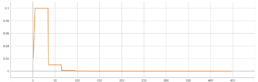
The graph below summarizes the improvements as we progressively built up our training recipe:
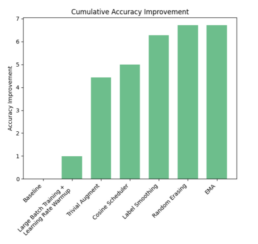
Using just a standard ResNet-50, we were able to achieve strong performance on the Stanford Cars dataset, demonstrating that careful tuning of a few simple techniques can go a long way in fine-grained classification.
However, it’s important to keep this in perspective. These results mainly show that we can train a model to distinguish between fine-grained, well-represented classes in a clean, curated dataset. The Stanford Cars dataset is nearly class-balanced, with high-quality, mostly frontal images and no major occlusion or real-world noise. It does not address challenges like long-tailed distributions, domain shift, or recognition of unseen classes.
In practice, you’ll never have a dataset that covers every car model—especially one that’s updated daily as new models appear. Real-world systems need to handle distributional shifts, open-set recognition, and imperfect inputs.
So while this served as a strong baseline and proof of concept, there was still significant work to be done to build something robust and production-ready.
References:
[1] Krause, Deng, et al. Collecting a Large-Scale Dataset of Fine-Grained Cars.
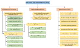
[2] Wei, et al. Fine-Grained Image Analysis with Deep Learning: A Survey.
[3] Reslan, Farou. Automatic Fine-grained Classification of Bird Species Using Deep Learning.
[4] Zhao, et al. A survey on deep learning-based fine-grained object clasiffication and semantic segmentation.
[5] He, et al. Bag of Tricks for Image Classification with Convolutional Neural Networks.
[6] Lee, et al. Compounding the Performance Improvements of Assembled Techniques in a Convolutional Neural Network.
[7] Wightman, et al. ResNet Strikes Back: An Improved Training Procedure in Timm.
[8] Vryniotis. How to Train State-of-the-Art Models Using TorchVision’s Latest Primitives.
[9] Krause et al, 3D Object Representations for Fine-Grained Catecorization.
[10] Müller, Hutter. TrivialAugment: Tuning-free Yet State-of-the-Art Data Augmentation.
[11] Zhong et al, Random Erasing Data Augmentation.