In the first part of this series, we built an intuition for generative modeling and placed diffusion models in the broader landscape of VAEs, GANs, and likelihood-based methods. We ended with a high-level idea: diffusion models gradually add Gaussian noise to data, step by step, and then learn to reverse that process.

The motivation for going all the way to noise is simple. If we can start from pure noise and reliably transform it into a realistic image, then we have a generative model. The forward noising process gives us a clean, well-defined starting point for sampling.

What’s less obvious is why this particular construction works.
Why does the noising happen gradually, instead of in a single step?
How does the model actually learn to denoise, and what training signal tells it that it is doing the right thing?
How does this correspond to learning a probability distribution at all?
Do we have mathematical guarantees that this process should work at all, rather than being a heuristic that just happens to work in practice?

These questions will be answered across the next two parts of the series. This second part is about setting up the necessary background. The third part will then focus entirely on diffusion models themselves. There, we will derive the forward noising process, the learned reverse dynamics, and the training objective in full detail. The goal here is not to memorize equations or reproduce derivations, but to build enough intuition to see the structure behind diffusion models. This is the level of understanding that lets you read papers, make sense of new variants as they appear, and reason about why certain design choices are made in the first place.

By the end of this part and the next, you should have a clear mental model for:

• why the forward noising process is constructed the way it is,

• why the reverse process can be learned at all,

• and how all of this connects to likelihood-based training.

With that foundation in place, we’ll be ready to implement our first diffusion model from scratch.

Much of the intuition and probabilistic framing in this part and the next, is adapted from [1] Calvin Luo, Understanding Diffusion Models: A Unified Perspective. This article selectively borrows from that work and focuses on building intuition rather than presenting full mathematical rigor. If you’re looking for a more complete and formal treatment, the original paper is exceptionally well written and highly recommended.

In Part 1, we explained that the goal of a generative model is to estimate the data density p(x). We also introduced latent variable models, where the observed data x is assumed to be generated with the help of unobserved latent variables z. In this setting, we can think of the model as described by a joint distribution: p(x,z).

Our goal is to learn the parameters of this distribution using the observed data. A natural approach is the Maximum Likelihood Estimation (MLE) we also presented in part 1, where we choose the parameters that maximize the likelihood of the observed data. The likelihood function measures the goodness of fit of a statistical model to a sample of data and it is formed from the joint probability distribution of the sample. Thus we want to to learn a model to maximize the likelihood p(x) of all observed x.

To connect the latent-variable model to the likelihood of the observed data, we marginalize out the latent variables:

We can also use the chain rule of probability:

Directly computing and maximizing this likelihood is difficult, because it requires integrating over all possible latent variables z or having access to the true posterior distribution p(z/x).  As discussed in Part 1, instead of maximizing the likelihood directly, we work with the log-likelihood,  also called the evidence. The log-likelihood is easier to work with mathematically, but the core problem remains: the marginalization over z is still intractable.

To address this, we introduce a quantity called the Evidence Lower Bound (ELBO). The equation of the ELBO is:

As its name suggests, the ELBO is a lower bound on the evidence:

Instead of optimizing the log-likelihood directly, we optimize a bound that we can work with. Maximizing the ELBO is a practical proxy with which to optimize a latent variable model.

Why is the Evidence Lower Bound (ELBO) a meaningful objective to optimize?

• Starting from Equation (1):
  \begin{equation} \begin{split} \log p(x) & = \log \int p(x,z) \,dz \\ & = \log \int \frac{p(x,z) q_{\phi}(z|x)}{q_{\phi}(z|x)}\\ & = \log{\mathbb{E}_{q_{\phi}(z|x)}\Biggl[\frac{p(x,z)}{q_{\phi}(z|x)}\Biggr]} \text{\quad \quad \quad \quad \quad (Definition of Expectation)}\\ & \geq \mathbb{E}_{q_{\phi}(z|x)}\Biggl[\log{\frac{p(x,z)}{q_{\phi}(z|x)}}\Biggr] \text{\quad \quad \quad \quad \quad (Jensen's Inequality)} \end{split} \end{equation}
• Using Equation 2:
  \begin{equation} \begin{split} \log{p(x)} & = \log{p(x)} \int q_{\phi}(z|x) \,dz \\ & = \int q_{\phi}(z|x) (\log{p(x)})\,dz \\ & = \mathbb{E}_{q_{\phi}(z|x)}[\log{p(x)}] \text{\quad \quad \quad \quad \quad \quad \quad \quad \quad \quad \quad \quad \quad \quad \quad (Definition of Expectation)}\\ & = \mathbb{E}_{q_{\phi}(z|x)}\Biggl[\log{\frac{p(x,z)}{p(z|x)}}\Biggl] \text{\quad \quad \quad \quad \quad \quad \quad \quad \quad \quad \quad \quad \quad (Equation 2)}\\ & = \mathbb{E}_{q_{\phi}(z|x)}\Biggl[\log{\frac{p(x,z)q_{\phi}(z|x)}{p(z|x)q_{\phi}(z|x)}}\Biggl]\\ & = \mathbb{E}_{q_{\phi}(z|x)}\Biggl[\log{\frac{p(x,z)}{q_{\phi}(z|x)}}\Biggl] + \mathbb{E}_{q_{\phi}(z|z)}\Biggl[\log{\frac{q_{\phi}(z|x)}{p(z|x)}}\Biggl]\\ & = \mathbb{E}_{q_{\phi}(z|x)}\Biggl[\log{\frac{p(x,z)}{q_{\phi}(z|x)}}\Biggl] + D_{KL}(q_{\phi}(z|x) \parallel p(z|x)) \text{\quad \quad (Definition of KL Divergence)}\\ & \geq \mathbb{E}_{q_{\phi}(z|x)}\Biggl[\log{\frac{p(x,z)}{q_{\phi}(z|x)}}\Biggl] \text{\quad \quad \quad \quad \quad \quad \quad \quad \quad \quad \quad \quad \, (KL Divergence always $\geq 0$)} \end{split} \end{equation}

The last equation tells us that the evidence (the log-likelihood) can be decomposed into two terms: the Evidence Lower Bound (ELBO) and the KL divergence between the approximate posterior and the true posterior.

What does this mean in practice?

Recall that we introduced the latent variable z to capture the underlying structure that explains the observed data x. Our original objective, is to find the parameters of the generative model, denoted by θ, that maximize the log-likelihood log⁡ p(x) but it is difficult since we don’t have access to the true posterior distribution p(z/x). To make progress, we introduced an approximation parameterized by Φ. We want to optimize the parameters of our approximation to exactly match the true posterior distribution.
The KL divergence measures how close this approximation is to the true posterior distribution. Minimizing the KL divergence corresponds exactly to making this approximation better. In the idealized case where our approximation is expressive enough and optimization succeeds perfectly, the KL divergence goes to zero.

The key point is that maximizing the ELBO plays two different roles. The evidence term is a constant with respect to the variational parameters Φ. Since the ELBO and the KL divergence sum to this constant, any increase in the ELBO must be accompanied by a corresponding decrease in the KL divergence. As a result, maximizing the ELBO with respect to Φ implicitly minimizes the KL divergence. With respect to the model parameters θ, however, the situation is different. The ELBO is a lower bound on the evidence. Therefore, maximizing the ELBO with respect to θ is equivalent to optimizing the evidence itself.

This variational perspective: introducing latent variables, approximating their posterior, and optimizing a lower bound on the data likelihood, is the conceptual foundation that we will later build upon

At the end of the previous section, we reached an important conclusion: one way to build a generative model with latent variables is to maximize the Evidence Lower Bound (ELBO) with respect to both the generative model parameters θ and the variational parameters ϕ. One model that relies on this idea is the variational autoencoder (VAE).
To understand VAEs, we need to address a subtle point that may not be intuitive to everyone: the posterior distribution is different for each data point x.

Consider a simple example. You observe the sum of two dice, which we call X, and the latent variable Z is the pair of individual dice values. If the observed sum is 2, the posterior distribution is trivial: the probability that both dice are 1 is 1, and the probability of any other outcome is 0. If the observed sum is 7, the posterior distribution is very different: several combinations such as (1,6), (2,5), and (3,4) all have non-zero probability. The shape of the distribution over latent variables depends entirely on the observed value of X.

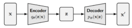
Because the posterior is different for every data point, in principle we would need a separate set of variational parameters ϕ for each individual x. The key idea behind variational autoencoders is to avoid this problem by learning an inference network. Instead of directly optimizing variational parameters for each data point, we train a neural network that takes x as input and outputs the parameters of the variational posterior. This network is trained jointly with the generative model. The generative model (often called the decoder) has parameters θ, while the inference network (can be interpreted as an encoder) has parameters ϕ. Both are optimized simultaneously by maximizing the ELBO.

Equation 7 dissects the ELBO term further, to make the connection explicit:

The two terms in this decomposition play complementary roles. The first term, encourages the model to learn latent variables that retain the information necessary to reconstruct the observed data. In other words, it ensures that the learned latent representation is meaningful. The second term measures how similar the learned variational distribution is to a prior belief held over latent variables. Maximizing the ELBO therefore amounts to maximizing its first term and minimizing its second term.

Once the inference network is trained, computing the posterior for a new data point is straightforward: we simply pass the data through the encoder network.

This architecture is called a variational autoencoder. It is autoencoder-like because data is mapped to a latent representation and then reconstructed back to itself through a bottleneck. It is variational because the latent representation is learned using variational inference. This probabilistic formulation encourages a smooth and continuous latent space, which is fundamentally different from the deterministic representations learned by standard autoencoders.

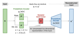
In practice, the encoder of a VAE is commonly chosen to model a multivariate Gaussian distribution with diagonal covariance, while the prior over latent variables is taken to be a standard multivariate Gaussian:

The KL divergence term of the ELBO can be computed analytically, and the first term can be approximated using a Monte Carlo estimate. Thus our objective can be rewritten as:

For each data point $x$ in the dataset, we sample latent variables \{z^{l}\}_{l=1}^{L} from the variational distribution q_{\phi}(z|x). However, this standard setup introduces a practical challenge: each z^{l}  is generated through a stochastic sampling process, which is not directly differentiable. As a result, it is not possible to optimize the model parameters using standard gradient-based methods.

This problem is addressed by the reparameterization trick when q_{\phi}(z|x) is designed to model certain distributions, including the multivariate Gaussian. The idea is to express a random variable as a deterministic transformation of a noise variable that is independent of the model parameters. This simple but powerful reformulation allows gradients to flow through the sampling process.
To see how the reparameterization trick works in practice, consider a simple example. Suppose we want to draw samples from a normal distribution with arbitrary mean and variance: x \sim \mathcal{N}(\mu, \sigma^2).

Instead of sampling x directly from this distribution, we can rewrite this as a deterministic transformation of a standard normal variable: x = \mu + \sigma \epsilon,  \text{with } \epsilon \sim \mathcal{N}(0, I).
Here, all the randomness is isolated in \epsilon, which is independent of the model parameters. The parameters \mu and \sigma now appear only in a deterministic transformation. This reformulation is mathematically equivalent to sampling from \mathcal{N}(\mu, \sigma^2), but it has a crucial practical advantage: gradients can flow through \muand \sigma during backpropagation.
In a variational autoencoder, the same idea is applied to the latent variable z. Recall that the encoder outputs the parameters of a Gaussian distribution: q_\phi(z \mid x) = \mathcal{N}\bigl(z; \mu_\phi(x), \sigma_\phi^2(x) I \bigr). Instead of sampling z directly from this distribution, we write: z = \mu_\phi(x) + \sigma_\phi(x) \odot \epsilon, \text{with } \epsilon \sim \mathcal{N}(0, I), where \odot denotes element-wise multiplication.

In this formulation, z is a deterministic function of the input x, the encoder parameters \phi, and an auxiliary noise variable \epsilon. The stochasticity is fully captured by \epsilon, which is independent of the network parameters. This allows us to compute gradients of the ELBO with respect to both \phiand \theta using standard gradient-based optimization.

The VAE therefore combines two key ideas:

• Monte Carlo estimation to approximate expectations, and

• the reparameterization trick to make those estimates differentiable.

After training, generation is straightforward. We sample directly from the prior over latent variables, z \sim p(z) and pass the sampled latent variable through the decoder. If training has succeeded, decoding samples from this simple Gaussian prior produces realistic data points in the original data space.

So far, we have studied the variational autoencoder as a latent variable model with a single layer of latent variables. We will now introduce an idea that generalizes this formulation. Instead of assuming that the data is generated from one latent variable, we allow multiple layers of latent variables, arranged hierarchically. In this setting, latent variables themselves are interpreted as generated from higher-level, more abstract latent variables. This leads to what is known as a Hierarchical Variational Autoencoder (HVAE).
In an HVAE with T hierarchical levels, each latent variable is, in general, allowed to condition on all previous latent variables in the hierarchy.
In this work, however, we focus on a particular structured case that we refer to as a Markovian Hierarchical VAE (MHVAE). In an MHVAE, the generative process forms a Markov chain. Each transition down the hierarchy is Markovian, meaning that decoding each latent variable z_t depends only on the latent variable directly above it, z_{t+1}. Intuitively, this structure can be viewed as stacking multiple VAEs on top of one another.

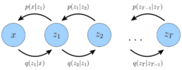
Mathematically, we represent the joint distribution and the posterior of a Markovian HVAE as:

Then, the ELBO can be extended to:

We can substitute the joint distribution (Equation 11) and the posterior (Equation 12) into Equation 16 to obtain an alternative form:

In this setting, generation becomes a sequential process: we sample from a simple prior at the top of the hierarchy and progressively transform it into data through a chain of conditional distributions. This perspective will turn out to be crucial, because diffusion models can be understood as a very particular instantiation of this framework.

In this article, we built the mathematical foundation necessary to understand diffusion models. We derived the Evidence Lower Bound (ELBO), explored variational autoencoders, and then generalized them to hierarchical and Markovian variational autoencoders. Along the way, we saw how maximizing the ELBO allows us to train generative models even when the true posterior is intractable.

In the next part, we will see that diffusion models are a very specific and carefully constructed instance of a Markovian Hierarchical VAE and the diffusion training objective will emerge naturally from the ELBO we derived here. Once that connection is fully clear, we will move from theory to practice. In Part 4, we will implement a diffusion model from scratch, translating every mathematical component into working PyTorch code. At that point, the entire picture will come together.

References:

[1] Calvin Luo. Understanding Diffusion Models: A Unified Perspective.

[2] Lilian Weng. From Autoencoder to Beta-VAE.

[3] Chieh-Hsin Lai et al. The Principles of Diffusion Models.